You segmented a plate. The pipeline worked. Now you have three label masks, a measurement file with 18,648 nuclei and tens of measurement columns, and a question: which of these cells actually responded?
The usual answer involves exporting tables, writing a notebook, and losing the one thing that matters most in imaging: the image. A scatter plot tells you that 7,531 objects fall below a threshold. It cannot show you which cells those are, sitting in their wells, next to their neighbors.
So we built the other answer into the Find Nuclei Viewer. Point it at your masks and measurements, and the plate becomes the plot.
Here is what that means. This is BBBC013 [1], 96 wells, exactly as the microscope saw it:
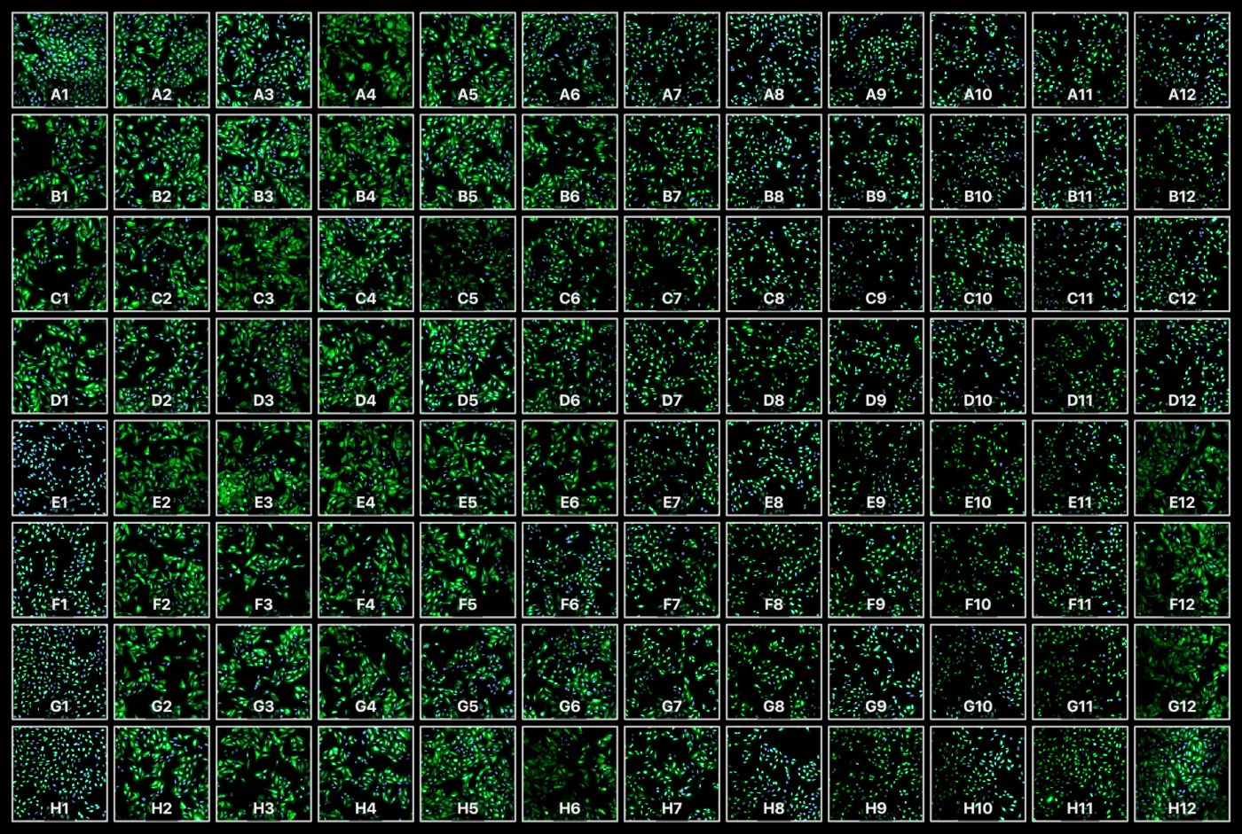
DRAQ (DNA) FKHR-GFP
And this is the same plate after segmentation and classification, every one of the 18,648 nuclei colored by its phenotype:
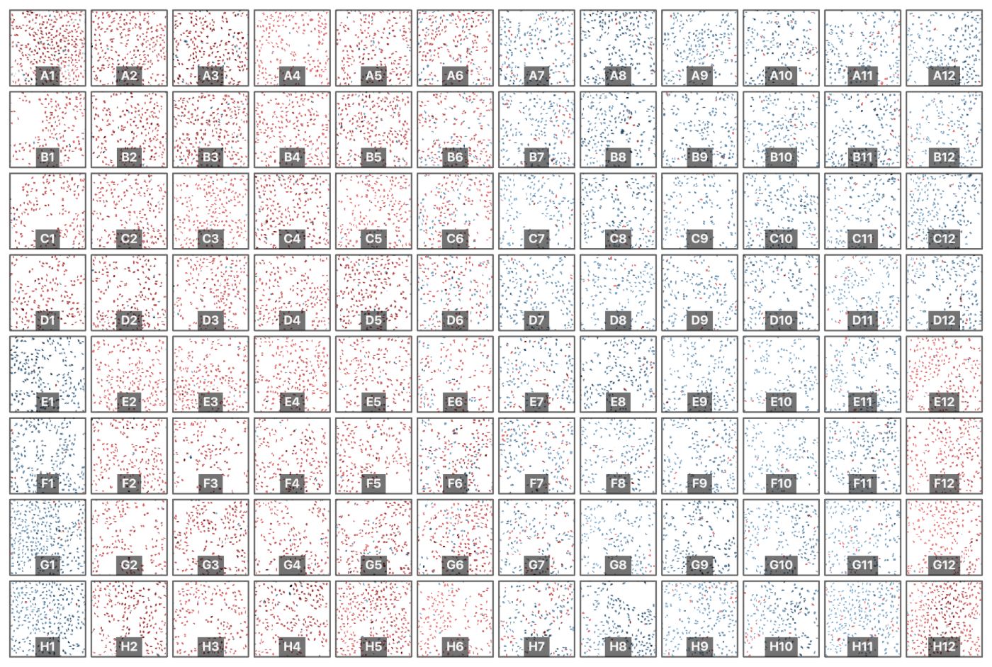
negative positive (translocated) excluded
The readout is visible before you open a single table: the left half of the plate stayed negative, the right half translocated. That gradient across the columns is the dose response. No export, no notebook, no plotting code. The image is the figure.
This is part one of a series on high-content screening. Today: what the viewer does with finished results. In part two, how those results get produced. Later, whole-slide images get the same treatment.
The setup
Everything below runs on BBBC013 [1] from the Broad Bioimage Benchmark Collection: human U2OS cells, a cytoplasm-to-nucleus translocation assay, 96 wells, two channels (DRAQ for DNA, FKHR-GFP). We ran StarDist [2] and Cellpose [3] over it to get nuclei, cell, and cytoplasm masks, then measured everything. That output is one folder containing masks and a measurment table.
The viewer reads that folder from a URL or straight from disk. Nothing is uploaded anywhere. Your browser fetches the chunks it needs and does the rest itself, which matters when the plate belongs to a client or is a part of a private study.
A note on the display, because neither plate above is a special export. The second one is the viewer’s inverted mode with the GFP channel switched off: dark nuclei on a white page, and nothing competing with the classification colors.
Color by any column
Every column in your table becomes a way to see the plate.
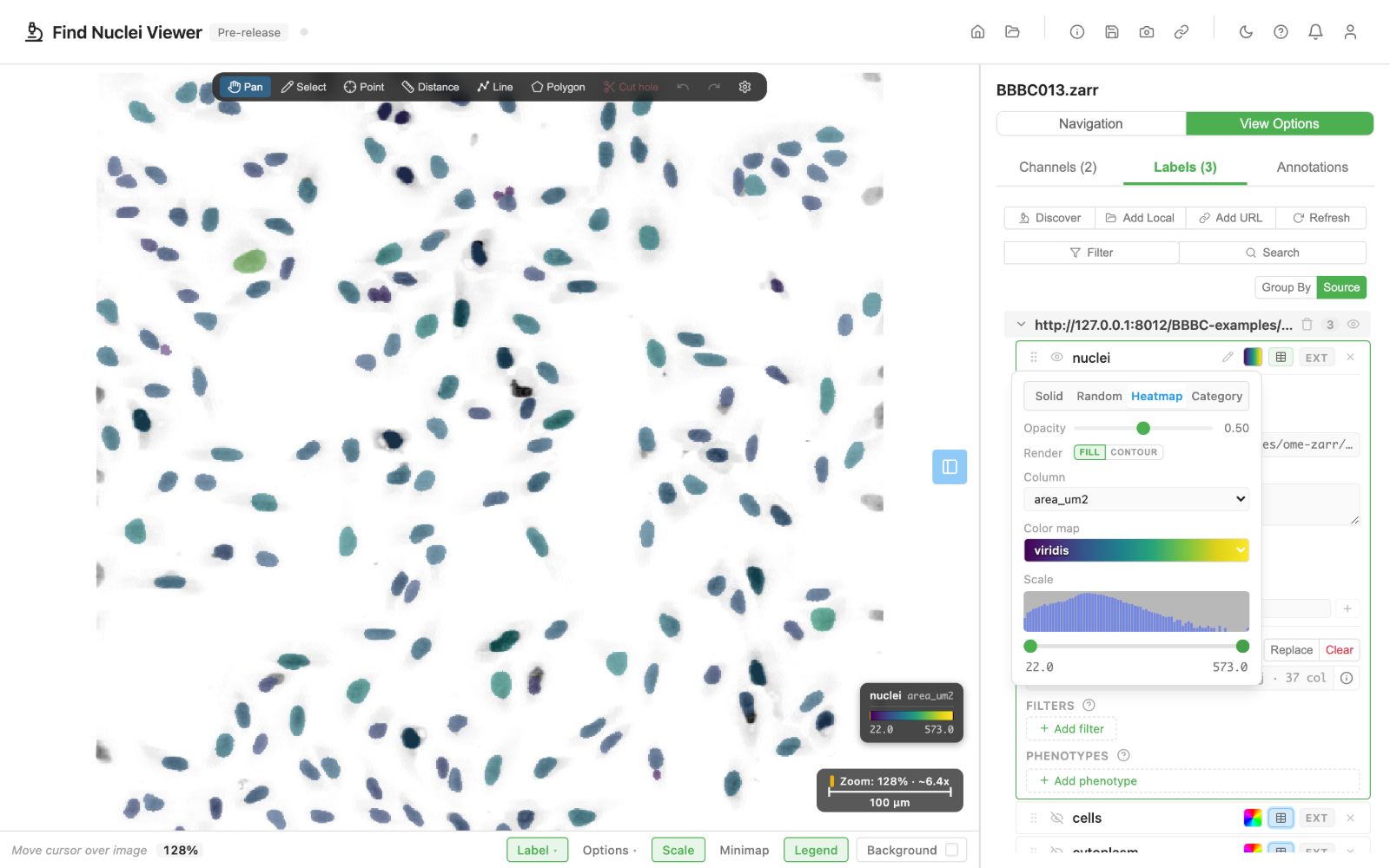
Pick a continuous measurement and you get a heatmap. Here the nuclei are colored by area, 22 to 573 square micrometers, and the outliers announce themselves immediately:
Pick a categorical column and each value gets its own color. Our pipeline wrote a phenotype_class column, so the translocation result is one click:
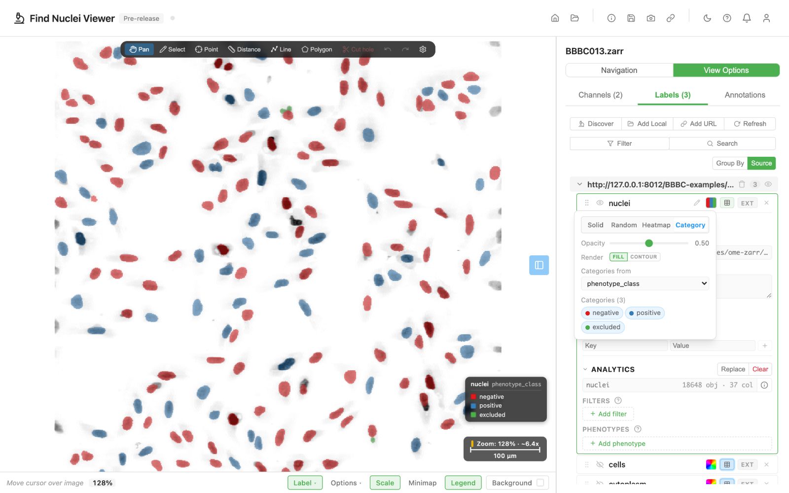
No plotting library, no export, no waiting. The colors are computed per object and drawn over the actual cells, so every “huh, that’s odd” is one zoom away from being investigated instead of being a dot in a scatter plot.
Filter until the question gets sharp
Filters hide objects that do not match. Drag a range on a histogram, or pick values from a list, and the plate updates as you drag. Multiple filters combine with AND: perimeter in this range, intensity above that, class equals positive.
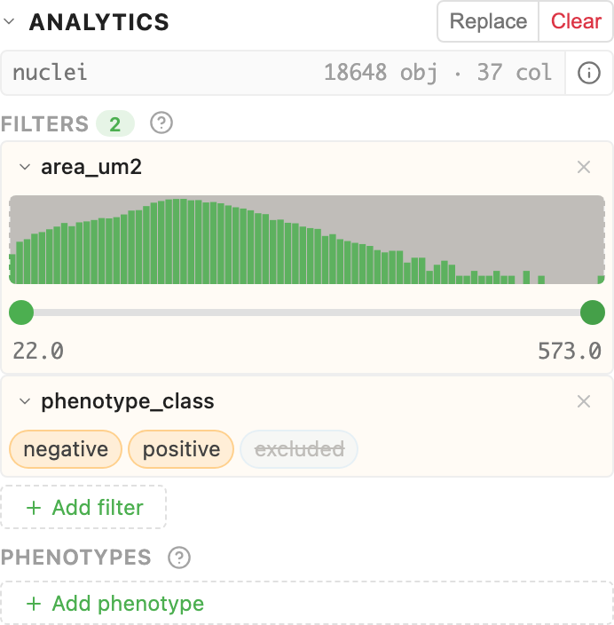
Filtering never changes the coloring. It answers a different question: not “what is this cell” but “which cells am I even looking at”.
Phenotypes: name the group, keep the gate
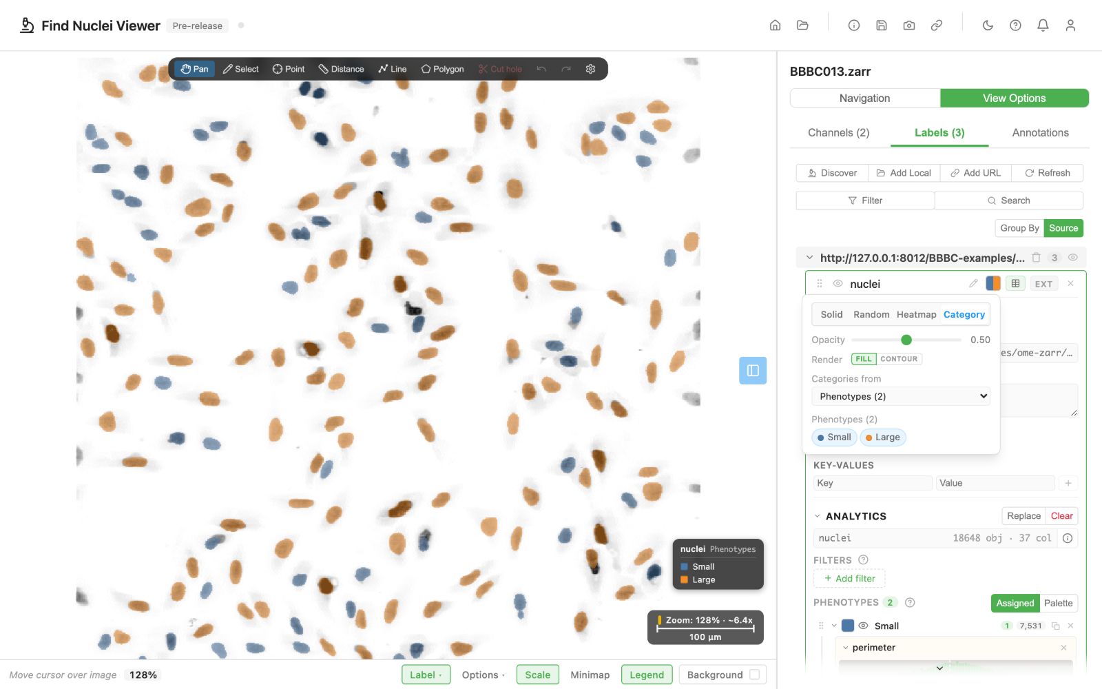
A phenotype is a named, colored group of filter conditions. Build one called Small with a perimeter gate, another called Large, and drag to reorder them; when an object matches several, the first match wins. It is gating, the flow-cytometry kind, except the gate draws itself on the image.
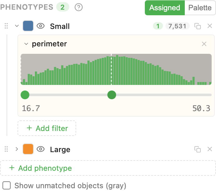
The counts update live. Move the slider, watch 7,531 become 7,214, and see exactly which cells changed their minds.
The part your pipeline will like
None of this depends on our tools having produced the data. The viewer reads a published, documented format: a directory with a manifest that names your masks and your measurements table. CSV works for a thousands of objects. Parquet streams column by column, so a 100-column table costs one small request until you actually color by something.
The whole format is documented, from a single CSV up to a multi-compartment analysis bundle, in the Analytics Data Format guide. If your pipeline can write a folder, it can feed this viewer.
The one rule that matters: the object ID in your table must equal the pixel value in your mask. That single convention is what makes the join a lookup instead of a spatial query, and it is what your segmentation tool already produces anyway.
Try it
The viewer is free to use and runs in any browser. Reading a dataset folder off your disk needs Chrome or Edge; a dataset zipped into a single .ozx or .zip file opens anywhere, Safari and Firefox included. The Analytics & Phenotyping guide walks through everything above with the same dataset, step by step.
Next in this series: where those masks and measurements came from, and how to go from a folder of raw plates to this view without writing glue code.
References
The segmentation masks and measurements shown are our output, not part of the original image collection.
[1] Ljosa V, Sokolnicki KL, Carpenter AE. Annotated high-throughput microscopy image sets for validation. Nature Methods 9(7), 637 (2012). https://bbbc.broadinstitute.org/BBBC013
[2] StarDist. https://github.com/stardist/stardist
[3] Cellpose. https://github.com/MouseLand/cellpose